<?xml version="1.0" encoding="utf-8"?><feed xmlns="http://www.w3.org/2005/Atom" ><generator uri="https://jekyllrb.com/" version="4.0.1">Jekyll</generator><link href="https://didarulislam.com/feed.xml" rel="self" type="application/atom+xml" /><link href="https://didarulislam.com/" rel="alternate" type="text/html" /><updated>2026-11-08T18:14:46+00:00</updated><id>https://didarulislam.com/feed.xml</id><title type="html">Didarul Islam</title><subtitle>This is my space where I share what I’m thinking about, learning, and building.</subtitle><author><name>Didarul Islam</name></author><entry><title type="html">Support Vector Machines from First Principles</title><link href="https://didarulislam.com/blog/2026/11/03/support-vector-machines/" rel="alternate" type="text/html" title="Support Vector Machines from First Principles" /><published>2026-11-03T00:00:00+00:00</published><updated>2026-11-03T00:00:00+00:00</updated><id>https://didarulislam.com/blog/2026/11/03/support-vector-machines</id><content type="html" xml:base="https://didarulislam.com/blog/2026/11/03/support-vector-machines/"><![CDATA[<p>Support Vector Machines (SVMs) were first proposed by Vladimir Vapnik and Alexey Chervonenkis in the mid-1960s and have since evolved into one of the most flexible and effective machine learning tools available <a class="citation" href="#chervonenkis2013early">[1]</a>. At their core, SVMs rest on some genuinely beautiful mathematics, and in this post, we’ll walk through it together in manageable pieces. This post aims to be self-contained: detailed enough that you can learn about the topic in its entirety without juggling multiple resources, yet concise enough so you can avoid the trap of minutiae.</p>

<p>Use the table of contents below to navigate the post:</p>

<ul>
  <li><a href="#1-hard-margin-svm">1 Hard-margin SVM</a>
    <ul>
      <li><a href="#1-1-intuition-of-margin">1.1 Intuition of margin</a></li>
      <li><a href="#1-2-optimal-margin-classifier">1.2 Optimal margin classifier</a></li>
    </ul>
  </li>
  <li><a href="#2-duality-of-svm">2 Duality of SVM</a>
    <ul>
      <li><a href="#2-1-primal-and-dual-problems">2.1 Primal and dual problems</a>
        <ul>
          <li><a href="#2-1-1-lagrangian">2.1.1 Lagrangian</a></li>
          <li><a href="#2-1-2-lagrange-dual-function">2.1.2 Lagrange dual function</a></li>
          <li><a href="#2-1-3-lagrange-dual-problem">2.1.3 Lagrange dual problem</a></li>
        </ul>
      </li>
      <li><a href="#2-2-weak-and-strong-duality">2.2 Weak and strong duality</a></li>
      <li><a href="#2-3-kkt-conditions">2.3 Karush-Kuhn-Tucker (KKT) conditions</a></li>
      <li><a href="#2-4-svm-dual-form">2.4 SVM dual form</a></li>
    </ul>
  </li>
  <li><a href="#3-kernels">3 Kernels</a>
    <ul>
      <li><a href="#3-1-feature-maps">3.1 Feature maps</a></li>
      <li><a href="#3-2-kernel-trick">3.2 Kernel trick</a></li>
      <li><a href="#3-3-the-kernelized-dual">3.3 The kernelized dual</a></li>
    </ul>
  </li>
  <li><a href="#4-regularized-svm">4 Regularized SVM</a>
    <ul>
      <li><a href="#4-1-slack-variables">4.1 Slack variables</a></li>
      <li><a href="#4-2-loss-function-form">4.2 Loss-function form</a></li>
      <li><a href="#4-3-subgradient-descent-method">4.3 Subgradient descent method</a></li>
    </ul>
  </li>
  <li><a href="#5-closing-thoughts">5 Closing thoughts</a></li>
</ul>

<div id="1-hard-margin-svm"></div>

<h2 id="1hard-margin-svm">1  Hard-margin SVM</h2>

<div id="1-1-intuition-of-margin"></div>

<h3 id="11intuition-of-margin">1.1  Intuition of margin</h3>
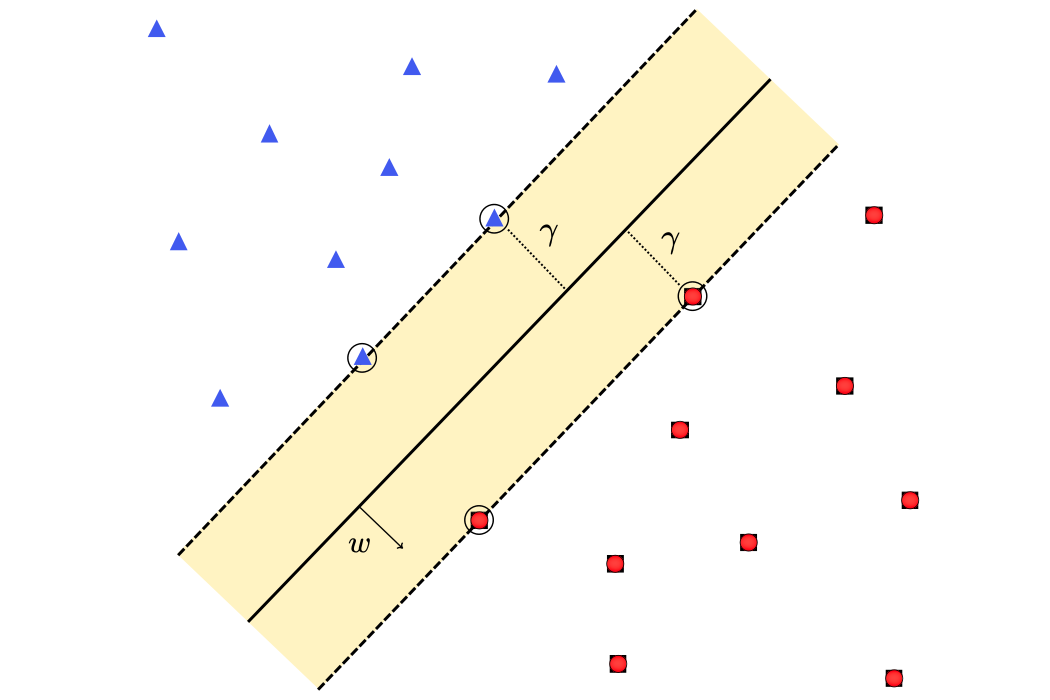
<p>Consider a training dataset \(\mathcal{D} = \big \{ (x_i, y_i) \big \}_{i=1}^M\), where $x_i \in \mathbb{R}^D$ is the $i$-th feature vector, and $y_i \in \{+1,-1\}$ is its binary label. A hyperplane splits this $D$-dimensional feature space into two half-spaces. If we assume (for now) that our dataset is linearly separable, there are infinitely many valid hyperplanes. We would like to estimate the optimal separating hyperplane that will correctly classify the two classes with the smallest classification error. The SVM prefers a hyperplane that does not favor any particular class. Geometrically, this corresponds to choosing a hyperplane that maximizes the distance between the hyperplane and the closest data points from both classes <a class="citation" href="#zaki2020datamining">[2]</a>. Intuitively, a hyperplane that scrapes right past our data is sensitive to small perturbations, while one with a wide buffer zone generalizes better.</p>

<figure class="figure-shrink">
  <img src="/assets/images/support-vector-machines/margin-intuition.svg" alt="Geometry of a linear SVM." />
<figcaption><strong>Figure 1:</strong> The separating hyperplane (solid) maximizes the margin $\gamma$ between the two classes. The support vectors (circled) from each class sit right on the edge of the margin.</figcaption>
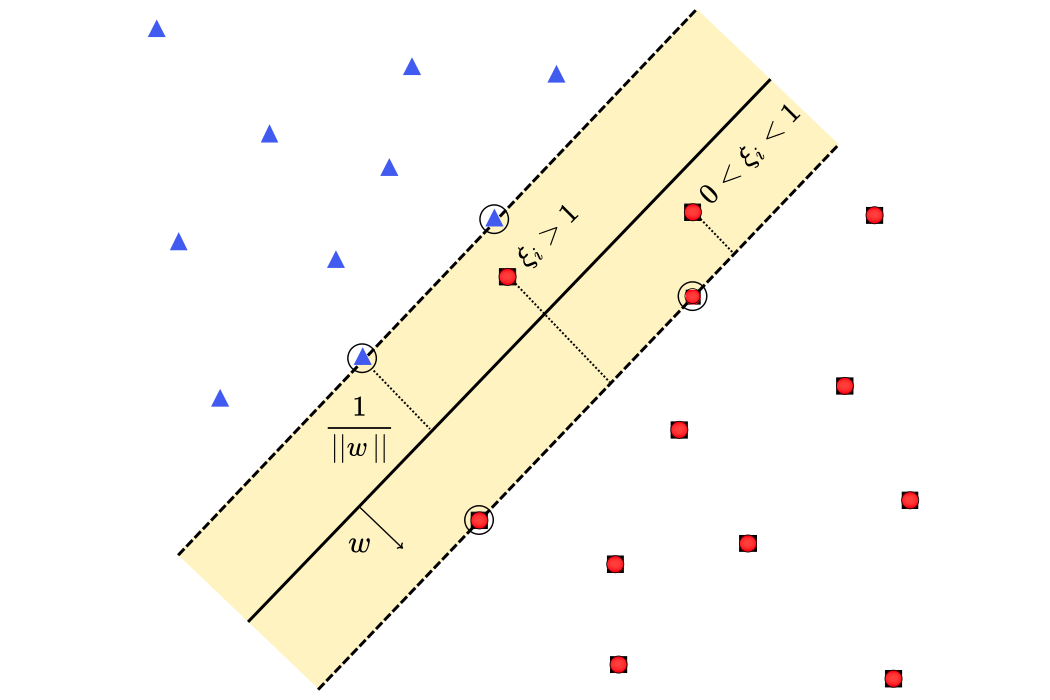
</figure>

<p>The data points that lie closest to the decision surface (or hyperplane) are called <em>support vectors</em>, and the distance from the hyperplane to the support vectors in either class defines the <em>margin</em>.</p>

<div id="1-2-optimal-margin-classifier"></div>

<h3 id="12optimal-margin-classifier">1.2  Optimal margin classifier</h3>

<p>In a $D$-dimensional space, a hyperplane is defined as follows:</p>

<div id="eq-1">
$$
\begin{align}
h(x) &amp;=w^Tx+b \tag{1}\\
&amp;=w_1x_1 + w_2x_2+ \cdots + w_Dx_D+b \notag
\end{align}
$$
</div>

<p>where $w \in \mathbb{R}^D$ is the normal vector orthogonal to the hyperplane, and $b \in \mathbb{R}$ is the bias term. For points lying on the hyperplane, we have</p>

<div id="eq-2">
$$
h(x)=w^Tx+b = 0  \tag{2}
$$
</div>

<p>Recall that a hyperplane $h(x)$ divides the original $D$-dimensional space into two half-spaces, such that every point labeled $y_i = +1$ satisfies $h(x_i) &gt; 0$, and every point labeled $y_i = -1$ satisfies $h(x_i) &lt; 0$. As such, the hyperplane $h(x)$ acts as a linear classifier that predicts the label $y$ of a point $x$ according to the following decision rule:</p>

<div id="eq-3">
$$
y = \begin{cases}
+1 &amp;\quad \text{if } h(x) &gt; 0 \tag{3}\\
-1 &amp;\quad \text{if }  h(x) &lt; 0
\end{cases}
$$
</div>

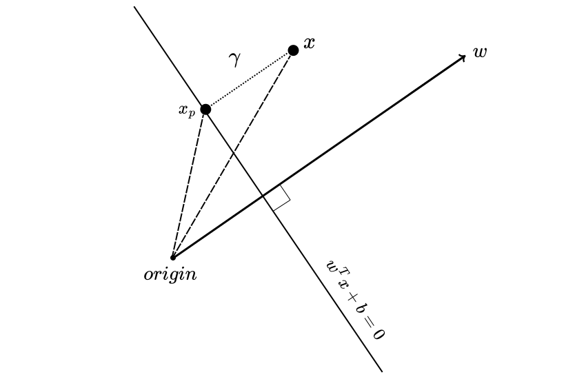
<p>Meanwhile, consider a point $x \in \mathbb{R}^D$ such that it does not lie on the hyperplane. Further let $x_p$ be the projection of $x$ onto the hyperplane along the normal vector $w$. Let $\gamma \gt 0$ be the distance from point $x$ to $x_p$ on the hyperplane.</p>

<figure class="figure-light">
  <img src="/assets/images/support-vector-machines/point-hyperplane-distance.svg" alt="Distance of a point to the hyperplane" />
<figcaption><strong>Figure 2:</strong> 
Illustration of the directed distance $\gamma$ from a point $x$ to the hyperplane.
</figcaption>
</figure>

<p>Since $w$ is the normal vector, the distance $\gamma$ is simply a scaling of $w$. Let’s assume that $w$ is of unit length $\lVert w \rVert = 1$, so following vector addition we can write:</p>

<div id="eq-4">
$$
x = x_p + \gamma \frac{w}{\lVert w \rVert} \tag{4}
$$
</div>

<p>Here $\gamma$ gives the <em>directed distance</em> of the point $x$ from $x_p$ in terms of the unit weight vector $\frac{w}{\lVert w \rVert}$. Note that $\gamma$ is positive when it points in the same direction as $w$, and negative when it points in the opposite direction.</p>

<p>Substituting Eq. <a href="#eq-4">(4)</a> into the hyperplane Eq. <a href="#eq-1">(1)</a> yields</p>

<div id="eq-5">
$$
\begin{align}
h(x) &amp;=  w^T(x_p + \gamma \frac{w}{\lVert w \rVert})+b  \notag\\
     &amp;= \underbrace{w^Tx_p + b}_{\text{0}} + \gamma \frac{w^Tw}{\lVert w \rVert} \notag \\
     &amp;= \gamma {\lVert w \rVert} \tag{5} \\
\end{align}
$$
</div>

<p>From Eq. <a href="#eq-5">(5)</a>, we can express the directed distance from the point to the hyperplane as</p>

<div id="eq-6">
$$
 \gamma = \frac {h(x)} {\lVert w \rVert} \tag{6} 
$$
</div>

<p>Since the distance must be nonnegative, we can multiply $\gamma$ by the point’s label $y$, which is $+1$ when $h(x) &gt; 0$ and $-1$ when $h(x)&lt;0$. Thus, the distance of a point $x$ from the hyperplane $h(x)$ is given as</p>

<div id="eq-7">
$$
\tilde{\gamma} = \frac{y h(x)}{\lVert w \rVert} \tag{7} 
$$
</div>

<p>Now, if we choose $x$ to be the point closest to the hyperplane, the distance $\tilde\gamma$ is the margin. We define the smallest distance between the hyperplane and all training points as</p>

<div id="eq-8">
$$
\gamma^{*} = \min_{i} {\tilde{\gamma}_i} = \min_{i}  \frac {y_i(w^T x_i + b)} {\lVert w \rVert} \tag{8} 
$$
</div>

<p>Note that scaling $w$ and $b$ in the hyperplane Eq. <a href="#eq-2">(2)</a> by the same constant $c&gt;0$ does not change the hyperplane. Hence, we scale $(w, b)$ by the <em>canonical normalization</em> such that</p>

<div id="eq-9">
$$
\min_{i}  y_i(w^T x_i + b) = 1 \tag{9} 
$$
</div>

<p>A support vector satisfies $y_i(w^T x_i + b)=1$, while any point that is not a support vector satisfies $y_i(w^T x_i + b) &gt; 1$. The geometric margin is $\gamma^{*} = \frac{1}{\lVert w \rVert}$ and the width of the margin band is $\frac{2}{\lVert w \rVert}$.</p>

<p>With the canonical normalization above, we can pose the following constrained optimization problem:</p>

<div id="eq-10">
$$
\max_{w,b} \; \gamma^{*} \quad \iff \quad \max_{w,b} \; \frac{1}{\lVert w \rVert} \tag{10} 
$$

$$
\text{s.t.}\quad y_i(w^T x_i + b) \ge 1,\quad \forall\, i=1,\ldots,M 
$$
</div>

<p>Maximizing the problem in Eq. <a href="#eq-10">(10)</a> is equivalent to minimizing the following problem:</p>

<div id="eq-11">
$$
\min_{w,b} \; {\lVert w \rVert}  \tag{11} 
$$

$$
\text{s.t.}\quad y_i​(w^Tx_i​+b)≥1, \quad \forall\, i=1,\ldots,M
$$
</div>

<p>Rather than minimizing the $l_2$-norm in Eq. <a href="#eq-11">(11)</a>, we often choose to minimize the squared norm because it yields a strictly convex quadratic objective. Thus, the new optimization problem becomes</p>

<div id="eq-12">
$$
\min_{w,b} \; {\lVert w \rVert}^2 \tag{12}
$$

$$
\text{s.t.}\quad y_i​(w^Tx_i​+b)≥1, \quad \forall\, i=1,\ldots,M 
$$
</div>

<p>The SVM formulation in Eq. <a href="#eq-12">(12)</a> is known as the <em>primal optimization problem</em>. The duality principle implies that an optimization problem may be viewed from either of two perspectives, the primal problem or the dual problem. In the next section, we will see how to transform the primal problem in Eq. <a href="#eq-12">(12)</a> into an equivalent <em>dual optimization problem</em>.</p>

<div id="2-duality-of-svm"></div>

<h2 id="2duality-of-svm">2.  Duality of SVM</h2>

<div id="2-1-primal-and-dual-problems"></div>

<h3 id="21primal-and-dual-problems">2.1  Primal and dual problems</h3>

<div id="2-1-1-lagrangian"></div>

<h4 id="211lagrangian">2.1.1  Lagrangian</h4>

<p>Consider a general optimization problem (the primal problem) defined as</p>

<div id="eq-13">
$$
\min_{x} \; f_0(x) \tag{13}
$$

$$
\text{s.t.}\quad f_i(x) \le 0,\quad \forall\, i=1,\ldots,M 
$$

$$
\qquad h_i(x) = 0,\quad \forall\, i=1,\ldots,P
$$
</div>

<p>where $x \in \mathbb{R}^N$ is the optimization variable, $f_0(x)$ is the objective function, $f_i(x) \le 0$ are $M$ inequality constraints, and $h_i(x) = 0$ are $P$ equality constraints.</p>

<p>The general idea in Lagrangian duality is to take the problem’s constraints into account by augmenting the objective function with a weighted sum of the constraint functions. We define the <em>Lagrangian</em> associated with the problem in Eq. <a href="#eq-13">(13)</a> as</p>

<div id="eq-14">
$$
\mathcal{L}(x,\alpha, \beta)= f_0(x) + \sum_{i=1}^{M}\alpha_if_i(x)+ \sum_{i=1}^{P}\beta_ih_i(x) \tag{14}
$$
</div>

<p>We refer to $\alpha_i$ as the <em>Lagrange multiplier</em> associated with the $i$-th inequality constraint $f_i(x) \le 0$, and $\beta_i$ as the Lagrange multiplier associated with the $i$-th equality constraint $h_i(x) = 0$.</p>

<p>The optimal value of the primal problem, denoted by $p^{*}$, is given by</p>

<div id="eq-15">
$$
p^* =  \inf_x  \sup_{\alpha \ge 0, \beta} \mathcal{L}(x,\alpha, \beta) \tag{15} 
$$
</div>

<div id="2-1-2-lagrange-dual-function"></div>

<h4 id="212lagrange-dual-function">2.1.2  Lagrange dual function</h4>

<p>Given a Lagrangian, we define its <em>Lagrange dual function</em> as</p>

<div id="eq-16">
$$
\begin{align}
g(\alpha, \beta) &amp;= \inf_x \mathcal{L}(x,\alpha, \beta)  \notag \\
                 &amp;= \inf_x \; \Biggl\{ f_0(x) + \sum_{i=1}^{M}\alpha_if_i(x)+ \sum_{i=1}^{P}\beta_ih_i(x) \Biggr\} \tag{16}
\end{align}
$$
</div>

<p>The Lagrange dual function is the pointwise infimum of a family of affine functions of $(\alpha, \beta)$, and thus it is concave even when the original problem in Eq. <a href="#eq-13">(13)</a> is nonconvex.</p>

<div id="2-1-3-lagrange-dual-problem"></div>

<h4 id="213lagrange-dual-problem">2.1.3  Lagrange dual problem</h4>

<p>Given the primal problem in Eq. <a href="#eq-13">(13)</a>, we define its <em>Lagrange dual problem</em> as</p>

<div id="eq-17">
$$
\max_{\alpha, \beta} \; g(\alpha, \beta) \tag{17}
$$

$$
\text{s.t.}\quad \alpha_i \ge 0, \quad \forall\, i=1,\ldots,M 
$$
</div>

<p>The optimal value of the dual problem, denoted by $d^{*}$, is given by</p>

<div id="eq-18">
$$
d^* =  \sup_{\alpha \ge 0, \beta}  \inf_x  \mathcal{L}(x,\alpha, \beta) \tag{18}
$$
</div>

<p>The dual problem is always a convex optimization problem since the objective to be maximized is concave and the constraint is convex <a class="citation" href="#boyd2004convex">[3]</a>. This is the case whether or not the primal problem in Eq. <a href="#eq-13">(13)</a> is convex.</p>

<div class="idea">
  <p class="note-title">📖 Terminology</p>
       <p>Concave maximization over a convex set is convex optimization.</p>
</div>

<div id="2-2-weak-and-strong-duality"></div>

<h3 id="22weak-and-strong-duality">2.2  Weak and strong duality</h3>

<p>The optimal value of the Lagrange dual problem $d^{*}$ gives us the <em>best lower bound</em> on the optimal value $p^{*}$ of the primal problem, i.e.,</p>

<div id="eq-19">
$$
d^{*} \le p^{*} \tag{19}
$$
</div>

<p>which holds for both convex and nonconvex problems. This property is called <em>weak duality</em>.</p>

<p>The difference $p^{*} - d^{*}$ is referred to as the <em>optimal duality gap</em>, which is always nonnegative <a class="citation" href="#boyd2004convex">[3]</a>. If the optimal duality gap is zero, then we say that strong duality holds, i.e.,</p>

<div id="eq-20">
$$
d^{*} = p^{*} \tag{20}
$$
</div>

<p>If strong duality holds, solving the dual is equivalent to solving the primal <a class="citation" href="#chiang2007optimization">[4]</a>. However, strong duality does not hold in general, but we usually (but not always) have strong duality if the primal problem is convex, i.e., of the form</p>

<div id="eq-21">
$$
\min_{x} \; f_0(x) \tag{21}
$$

$$
\begin{align}
\text{s.t.}\quad &amp; f_i(x) \le 0,\quad \forall\, i=1,\ldots,M   \notag \\
                 &amp; Ax=b  \notag
\end{align}
$$
</div>

<p>where $f_0, \ldots, f_M$ are convex functions. Beyond convexity, the conditions which guarantee strong duality are called <em>constraint qualifications</em>.</p>

<div class="note">
  <p class="note-title">📝 Note</p>
  <span>Convexity</span> + <span>Constraint Qualifications</span> ⟹ Strong Duality
</div>

<p>One simple but well-known constraint qualification is <em>Slater’s condition</em>: there exists an $x \in \operatorname{relint} D$ such that</p>

<div id="eq-22">
$$
f_i(x) &lt; 0, \quad \forall\, i=1,\ldots,M,  \quad Ax=b \tag{22}
$$
</div>

<p>Such a point is often referred to as <em>strictly feasible</em>, since the inequality constraints hold with strict inequalities. Slater’s theorem states that strong duality holds if Slater’s condition holds and the optimization problem is convex.</p>

<p>Slater’s condition in Eq. <a href="#eq-22">(22)</a> can be refined when some of the inequality constraint functions $f_i$ are affine. If the first $K$ constraint functions $f_1, \ldots, f_K$ are affine, then strong duality holds provided the following weaker condition holds: there exists an $x \in \operatorname{relint} D$ with</p>

<div id="eq-23">
$$
f_i(x) \le 0, \quad \forall\, i=1,\ldots,K,  \qquad f_i(x) &lt; 0, \quad \forall\, i=K+1,\ldots,M, \qquad Ax=b \tag{23}
$$
</div>

<p>Detailed proof of the Slater’s theorem can be found in Boyd and Vandenberghe’s <a href="https://stanford.edu/~boyd/cvxbook/bv_cvxbook.pdf" target="_blank" rel="noopener noreferrer"><em>Convex Optimization</em></a> book (see Sec. 5.3.2, pp. 234-236).</p>

<div id="2-3-kkt-conditions"></div>

<h3 id="23karush-kuhn-tucker-kkt-conditions">2.3  Karush-Kuhn-Tucker (KKT) conditions</h3>

<p><strong>For general problems:</strong> for an optimization problem with differentiable objective and constraint functions, if strong duality holds, any pair of primal and dual optimal points must satisfy the following KKT conditions:</p>

<div id="eq-24">
$$
\begin{align}
f_i(x) &amp;\le 0, &amp;&amp;\forall\, i = 1,\ldots,M \tag{24}\\
h_i(x) &amp;= 0, &amp;&amp;\forall\, i = 1,\ldots,P \tag{25}\\
\alpha_i &amp;\ge 0, &amp;&amp;\forall\, i = 1,\ldots,M \tag{26}\\
\alpha_i f_i(x) &amp;= 0, &amp;&amp;\forall\, i = 1,\ldots,M \tag{27}\\
\nabla f_0(x) + \sum_{i=1}^{M}\alpha_i\nabla f_i(x) + \sum_{i=1}^{P}\beta_i\nabla h_i(x) &amp;= 0 \tag{28}
\end{align}
$$
</div>

<p><strong>For convex problems:</strong> for a convex optimization problem with differentiable objective and constraint functions, any points that satisfy the KKT conditions are primal and dual optimal, and have zero duality gap, i.e., $p^{*}=d^{*}$.</p>

<p><strong>For convex problems satisfying Slater’s condition:</strong> for a convex optimization problem with differentiable objective and constraint functions that satisfies Slater’s condition, the KKT conditions provide necessary and sufficient conditions for optimality.</p>

<div id="2-4-svm-dual-form"></div>

<h3 id="24svm-dual-form">2.4  SVM dual form</h3>

<p>Let’s revisit the primal SVM formulation in Eq. <a href="#eq-12">(12)</a>, which can be equivalently expressed as the following constrained problem:</p>

<div id="eq-29">
$$
\min_{w,b} \; \frac{1}{2}{\lVert w \rVert}^2 \tag{29}
$$

$$
\text{s.t.}\quad -y_i​(w^Tx_i​+b) + 1\le 0, \quad \forall\, i=1,\ldots,M
$$
</div>

<p>where we introduce a constant $\frac{1}{2}$, which does not affect the optimal $w, b$ but simplifies our later derivations. This is a differentiable, convex optimization problem that satisfies Slater’s condition; therefore, strong duality $(p^{*}=d^{*})$ holds, and the KKT conditions are necessary and sufficient for optimality.</p>

<p>We first define the Lagrangian of the primal SVM problem as</p>

<div id="eq-30">
$$
\mathcal{L}(w,b,\alpha) = \frac{1}{2}{\lVert w \rVert}^2 - \sum_{i=1}^{M}\alpha_iy_i​(w^Tx_i​+b) + \sum_{i=1}^{M}\alpha_i \tag{30}
$$
</div>

<p>Recall that the Lagrange dual function can be formulated as</p>

<div id="eq-31">
$$
\begin{align}
g(\alpha) &amp;= \inf_{w,b} \mathcal{L}(w, b,\alpha)  \notag \\
                 &amp;= \inf_{w,b} \; \Biggl\{ \frac{1}{2}{\lVert w \rVert}^2 - \sum_{i=1}^{M}\alpha_iy_i​(w^Tx_i​+b) + \sum_{i=1}^{M}\alpha_i  \Biggr\} \tag{31}
\end{align}
$$
</div>

<p>In order to obtain the extremum of the Lagrangian with respect to $w$ and $b$, we compute the gradient of $\mathcal{L}(w,b,\alpha)$ with respect to $w$ and $b$, and set them to zero,</p>

<div id="eq-32">
$$
\nabla_w \mathcal{L}(w,b,\alpha) =  w - \sum_{i=1}^{M}\alpha_iy_i​x_i = 0 \tag{32}
$$
</div>

<p>and we thus have</p>

<div id="eq-33">
$$
w = \sum_{i=1}^{M}\alpha_iy_i​x_i \tag{33} 
$$
</div>

<p>Similarly,</p>

<div id="eq-34">
$$
\frac{\partial\mathcal{L}}{\partial b}(w,b,\alpha) = \sum_{i=1}^{M}\alpha_iy_i​ = 0 \tag{34} 
$$
</div>

<p>Plugging Eq. <a href="#eq-33">(33)</a> and Eq. <a href="#eq-34">(34)</a> into Eq. <a href="#eq-31">(31)</a>, we get</p>

<div id="eq-35">
$$
g(\alpha) = \inf_{w,b}  \mathcal{L}(w,b,\alpha)  = \sum_{i=1}^{M}\alpha_i - \frac{1}{2}\sum_{i=1}^{M}\sum_{j=1}^{M}\alpha_i\alpha_j y_i y_j (x_i^T x_j) \tag{35} 
$$
</div>

<p>Hence, the dual problem can be written as</p>

<div id="eq-36">
$$
\max_{\alpha} \; g(\alpha) = \sum_{i=1}^{M}\alpha_i - \frac{1}{2}\sum_{i=1}^{M}\sum_{j=1}^{M}\alpha_i\alpha_j y_i y_j (x_i^T x_j) \tag{36}
$$

$$
\text{s.t.}\quad \begin{cases}
\alpha_i \ge 0, \quad \forall\, i = 1, \ldots, M \\
\displaystyle\sum_{i=1}^{M} \alpha_i y_i = 0
\end{cases}
$$
</div>

<p>This is a convex quadratic programming (QP) problem that can be efficiently solved with the <a href="https://www.microsoft.com/en-us/research/wp-content/uploads/1998/04/sequential-minimal-optimization.pdf" target="_blank" rel="noopener noreferrer"><em>Sequential Minimal Optimization (SMO)</em></a> algorithm. Exactly how to solve such a QP problem is beyond the scope of this post. The dual optimization problem is introduced here mainly because it is easy to <em>kernelize</em>.</p>

<p>However, recall that according to the KKT condition in Eq. <a href="#eq-24">(27)</a>, we have</p>

<div id="eq-37">
$$
\alpha_i(-y_i​(w^Tx_i​+b) + 1) = 0 \tag{37}
$$
</div>

<p>which gives rise to two scenarios:</p>

<ul>
  <li>$\alpha_i = 0$, or</li>
  <li>$y_i​(w^Tx_i​+b) = 1$</li>
</ul>

<p>This is a very important insight, since if $\alpha_i &gt; 0$, then $y_i​(w^Tx_i​+b) = 1$, i.e., the training data points $x_i$ whose $\alpha_i$’s are nonzero are the support vectors. Once we have the Lagrange multipliers $\{\alpha_i\}$, we can reconstruct the weight vector $w$ as a linear combination of support vectors</p>

<div id="eq-38">
$$
w = \sum_{i \in \mathcal{S}}\alpha_iy_i​x_i \tag{38} 
$$
</div>

<p>where $\mathcal{S}$ denotes the set of the indices of the support vectors. This “sparse” representation is advantageous for making new predictions since the final classifier depends only on the small subset of data points $x_i$ with $\alpha_i &gt; 0$, i.e., the support vectors.</p>

<p><strong>SVM Classifier:</strong> For any new point $z$, we predict the class as</p>

<div id="eq-39">
$$\begin{align}
\hat{y}&amp;=\operatorname{sign}​(w^Tz​+b) \notag\\
\hat{y}&amp;=\operatorname{sign}​\biggl(\sum_{i \in \mathcal{S}}\alpha_iy_i(​x_i^Tz​)+b\biggr) \tag{39}
\end{align}
$$
</div>

<p>where the $\operatorname{sign}$(·) function returns $+1$ for any positive argument, and $-1$ for any negative argument.</p>

<div id="3-kernels"></div>

<h2 id="3kernels">3  Kernels</h2>

<div id="3-1-feature-maps"></div>

<h3 id="31feature-maps">3.1  Feature maps</h3>

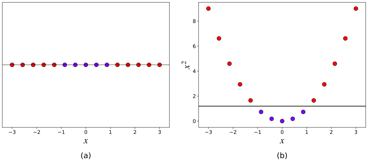
<p>Imagine a binary classification problem as shown in Fig. <a href="#Fig-3">3(a)</a>. Each data sample is represented by a single feature $x \in \mathbb{R}$, and the dataset cannot be separated by a linear hyperplane. How can we extend the linear SVM model to solve such a nonlinear problem?</p>

<p>To make life easier, we can transform each data sample to a higher-dimensional feature space where it is more likely to exhibit linear patterns. In our classification problem, for example, we map each sample from the $1$-dimensional input space into a $2$-dimensional feature space via the feature mapping:</p>

<div id="eq-40">
$$
\phi: \mathbb{R} \rightarrow \mathbb{R}^2, \quad x \mapsto \begin{bmatrix}x \\ x^2\end{bmatrix} \tag{40}
$$ 
</div>

<p>where $\phi$ is a feature map, which maps the original input attributes to the features. As shown in Fig. <a href="#Fig-3">3(b)</a>, each sample now has two features, and we can find a linearly separable hyperplane in the new feature space.</p>

<div id="Fig-3">
<figure class="figure-wide">
  <img src="/assets/images/support-vector-machines/feature-mapping.svg" alt="Mapping nonseparable 1D data to a linearly separable higher-dimensional feature space." />
  <figcaption><strong>Figure 3:</strong>
    (a) The data samples lie in a $1$-dimensional input space. (b) The data samples become linearly separable in the new higher-dimensional feature space.
  </figcaption>
</figure>
</div>

<p>The idea of “lifting” our data into a higher-dimensional space is very cool. However, feature mapping usually causes the number of features to blow up! Explicitly constructing such a mapping is computationally inefficient, especially when the new feature space is very high-dimensional <a class="citation" href="#li_svm_notes">[5]</a>. Fortunately, the kernel trick comes to the rescue.</p>

<div id="3-2-kernel-trick"></div>

<h3 id="32kernel-trick">3.2  Kernel trick</h3>

<p>Let’s rewrite the SVM formulation in Eq. <a href="#eq-36">(36)</a> by replacing the original input attributes $x$ with a feature map $\phi(x)$:</p>

<div id="eq-41">
$$
\begin{align}
\max_{\alpha} \; &amp; \sum_{i=1}^{M}\alpha_i - \frac{1}{2}\sum_{i=1}^{M}\sum_{j=1}^{M}\alpha_i\alpha_j y_i y_j \langle\phi(x_i), \phi(x_j)\rangle \tag{41} \\
\text{s.t.}\quad &amp; \begin{cases}
\alpha_i \ge 0, \quad \forall\, i = 1, \ldots, M \notag\\
\displaystyle\sum_{i=1}^{M} \alpha_i y_i = 0
\end{cases}
\end{align}
$$
</div>

<p>where $\phi(x_i)^T \phi(x_j)$ is equivalently written as $\langle\phi(x_i), \phi(x_j)\rangle$, emphasizing the inner product of the two feature vectors.</p>

<div id="Fig-4">
<figure class="figure-wide">
  <img src="/assets/images/support-vector-machines/polynomial-mapping-3D.svg" alt="Polynomial kernel makes the data linearly separable in 3D." />
  <figcaption><strong>Figure 4:</strong>
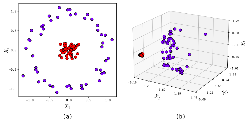
    (a) Data is not linearly separable in the $2$-dimensional input space. (b) Linearly separable data in the $3$-dimensional feature space after a degree-$2$ polynomial transformation.
  </figcaption>
</figure>
</div>

<p>Now let’s look at another classic binary classification problem as shown in Fig. <a href="#Fig-4">4(a)</a>. We are working with $2$-dimensional data samples that are not linearly separable in the input space. Each data sample is represented by</p>

<div id="eq-42">
$$
x = \begin{bmatrix}
x_1 \\
x_2
\end{bmatrix} \tag{42}
$$
</div>

<p>For a <a href="https://en.wikipedia.org/wiki/Polynomial_kernel" target="_blank" rel="noopener noreferrer"><em>polynomial kernel</em></a> of degree $2$, the corresponding feature map $\phi$ is given by</p>

<div id="eq-43">
$$
\phi: \mathbb{R}^2 \rightarrow \mathbb{R}^3, \quad \begin{bmatrix} x_1 \\ x_2 \end{bmatrix} \mapsto \begin{bmatrix} {x_1}^2 \\[3pt] {x_2}^2 \\[3pt] {\sqrt{2}x_1x_2} \end{bmatrix}\tag{43}
$$ 
</div>

<p>The inner product in the feature space is</p>

<div id="eq-44">
$$
\begin{align}
\phi(x_i)^T\phi(x_j)
&amp;=
\begin{bmatrix}x_{i,1}^{2} &amp; x_{i,2}^{2} &amp; \sqrt{2}\,x_{i,1}x_{i,2}\end{bmatrix}
\begin{bmatrix}x_{j,1}^{2}\\[6pt] x_{j,2}^{2}\\[6pt] \sqrt{2}\,x_{j,1}x_{j,2} \end{bmatrix} \notag \\[6pt]
&amp;=x_{i,1}^{2}x_{j,1}^{2}+x_{i,2}^{2}x_{j,2}^{2}+2x_{i,1}x_{i,2}x_{j,1}x_{j,2} \tag{44} 
\end{align}
$$
</div>

<p>Now consider a <em>kernel function</em> $k$ in a $2$-dimensional input space defined as follows:</p>

<div id="eq-45">
$$
k(x_i,x_j) = (x_i^T x_j)^2 \tag{45}
$$
</div>

<p>Expanding it gives</p>

<div id="eq-46">
$$
\begin{align}
k(x_i,x_j) &amp;=\biggl(\begin{bmatrix}x_{i,1} &amp; x_{i,2}\end{bmatrix}\begin{bmatrix} x_{j,1}\\[6pt] x_{j,2}\\[6pt] \end{bmatrix}\biggr)^2 \notag\\[6pt]
&amp;=(x_{i,1}x_{j,1}+x_{i,2}x_{j,2})^2 \notag\\[6pt]
&amp;=x_{i,1}^{2}x_{j,1}^{2}+x_{i,2}^{2}x_{j,2}^{2}+2x_{i,1}x_{i,2}x_{j,1}x_{j,2} \notag\\[6pt]
&amp;=\phi(x_i)^T\phi(x_j) \tag{46}
\end{align}
$$
</div>

<p>Did you notice what just happened? We just demonstrated that through the kernel function $k(x_i,x_j)$ we can implicitly compute the inner product $\langle\phi(x_i), \phi(x_j)\rangle$ directly from the original input space rather than constructing the explicit feature mapping. This is known as the <strong>kernel trick</strong>. The key advantage of the kernel trick is computational efficiency.</p>

<p>An example would help this make more sense.</p>

<p>Let</p>

<div id="eq-47">
$$
x_i = \begin{bmatrix}
1 \\
2
\end{bmatrix},
\qquad
x_j = \begin{bmatrix}
3 \\
4
\end{bmatrix}
\tag{47}
$$
</div>

<p>and its corresponding inner product in the feature space is</p>

<div id="eq-48">
$$
\begin{align}
\phi(x_i)^T\phi(x_j)
&amp;=
\begin{bmatrix} (1)^2 &amp; (2)^2 &amp; \sqrt{2} \cdot (1 \cdot 2) \end{bmatrix}
\begin{bmatrix}(3)^2 \\[6pt] (4)^2 \\[6pt] \sqrt{2} \cdot (3 \cdot 4) \end{bmatrix} \notag \\[6pt]
&amp;=(1 \cdot 1) \cdot (3 \cdot 3) + (2 \cdot 2) \cdot (4 \cdot 4) + \sqrt{2} \cdot (1 \cdot 2) \cdot \sqrt{2} \cdot (3 \cdot 4) \notag\\[6pt]
&amp;= 9+64+48 \notag\\[6pt]
&amp;=121 \tag{48}
\end{align}
$$
</div>

<p>Explicitly constructing both feature vectors and then taking their inner product requires 13 operations (11 multiplications, 2 additions).</p>

<p>Now consider direct kernel evaluation:</p>

<div id="eq-49">
$$
\begin{align}
k(x_i,x_j) &amp;=\biggl(\begin{bmatrix}1 &amp; 2\end{bmatrix}\begin{bmatrix} 3\\[6pt] 4\\[6pt] \end{bmatrix}\biggr)^2 \notag\\[6pt]
&amp;=(1 \cdot 3 + 2 \cdot 4)^2 \notag\\[6pt]
&amp;=11 \cdot 11 \notag\\[6pt]
&amp;=121 \tag{49}
\end{align}
$$
</div>

<p>Direct kernel evaluation requires only 4 operations (3 multiplications, 1 addition). In other words, a suitable kernel function cheaply computes the inner product $\langle\phi(x_i), \phi(x_j)\rangle$ in the feature space without the lifting.</p>

<p>Let’s formalize the concept of a kernel function. Let $\mathcal{X}$ denote an input space. A function $k:\mathcal{X} \times \mathcal{X} \rightarrow \mathbb{R}$ is a <strong>kernel function</strong> over $\mathcal{X}$ if there exist a real Hilbert space $\mathcal{H}$ and a feature map $\phi:\mathcal{X} \rightarrow \mathcal{H}$ such that</p>

<div id="eq-50">
$$
k(x_i,x_j) = {\langle \phi(x_i), \phi(x_j) \rangle}, \quad \forall \ x_i,x_j \in \mathcal{X} \tag{50}
$$
</div>

<p>where $\langle \cdot,\cdot \rangle$ denotes the inner product on $\mathcal{H}$.</p>

<p>But can any function be used as a kernel function? The answer is no. Not every function is a valid kernel. <em>Mercer’s theorem</em> provides the theoretical foundation for characterizing valid kernels (see <a href="https://people.eecs.berkeley.edu/~jordan/courses/281B-spring04/lectures/lec3.pdf" target="_blank" rel="noopener noreferrer"><em>Michael Jordan’s lecture notes</em></a>). However, note that Mercer’s theorem only tells us whether a candidate similarity function is admissible for use as a kernel, not how well it would perform <a class="citation" href="#chandrasekaran2025kernel">[6]</a>.</p>

<p>Some common kernels include:</p>

<ul>
  <li><strong>Linear Kernel:</strong> $k(x_i,x_j) = \langle x_i, x_j \rangle = x_i^Tx_j$. This is the simplest kernel. It applies no feature mapping and is equivalent to the standard linear SVM.</li>
  <li><strong>Polynomial Kernel:</strong> $k(x_i,x_j) = (\gamma  \langle x_i, x_j \rangle + r)^{d}$, where $\gamma \gt 0$ is a scale factor, $r$ is a constant term, and $d$ is the degree of the polynomial. In our example in Eq. <a href="#eq-45">(45)</a>, the values are $\gamma = 1$, $r = 0$, and $d = 2$.</li>
  <li><strong>Radial Basis Function (RBF) Kernel:</strong> $k(x_i,x_j) = \exp (-\gamma {\lVert x_i - x_j \rVert}^2)$, where $\gamma \gt 0$ is a scale factor. The RBF kernel is also called the Gaussian kernel and is a popular default choice for nonlinear problems.</li>
  <li><strong>Sigmoid Kernel:</strong> $k(x_i,x_j) = \tanh (\gamma  \langle x_i, x_j \rangle + r)$. This kernel is inspired by the activation function used in neural networks.</li>
</ul>

<div id="3-3-the-kernelized-dual"></div>

<h3 id="33the-kernelized-dual">3.3  The kernelized dual</h3>

<p>Now let’s reformulate the dual problem in Eq. <a href="#eq-41">(41)</a> by replacing the inner product $\langle\phi(x_i), \phi(x_j)\rangle$ with a kernel function $k(x_i,x_j)$:</p>

<div id="eq-51">
$$
\begin{align}
\max_{\alpha} \; &amp; \sum_{i=1}^{M}\alpha_i - \frac{1}{2}\sum_{i=1}^{M}\sum_{j=1}^{M}\alpha_i\alpha_j y_i y_j k(x_i,x_j) \tag{51} \\
\text{s.t.}\quad &amp; \begin{cases}
\alpha_i \ge 0, \quad \forall\, i = 1, \ldots, M \notag\\
\displaystyle\sum_{i=1}^{M} \alpha_i y_i = 0
\end{cases}
\end{align}
$$
</div>

<p>This reformulation is what allows SVMs to learn a linear decision boundary in feature space, which corresponds to a nonlinear decision boundary in the original input space.</p>

<p><strong>Classifier:</strong> For any new point $z$, the predicted class can be expressed in terms of the kernel:</p>

<div id="eq-52">
$$\begin{align}
\hat{y}&amp;=\operatorname{sign}​(\langle w, \phi(z) \rangle ​+b) \notag\\
&amp;=\operatorname{sign}​\biggl(\sum_{i \in \mathcal{S}}\alpha_iy_i \langle \phi(​x_i),\phi(z​) \rangle +b\biggr) \notag \\
&amp;=\operatorname{sign}​\biggl(\sum_{i \in \mathcal{S}}\alpha_iy_i k(x_i,z) +b\biggr) \tag{52}
\end{align}
$$
</div>

<div id="4-regularized-svm"></div>

<h2 id="4regularized-svm">4  Regularized SVM</h2>

<div id="4-1-slack-variables"></div>

<h3 id="41-slack-variables">4.1 Slack variables</h3>

<p>So far, we’ve seen that when a dataset cannot be separated by a hyperplane, we can use kernels to implicitly map the data to a higher-dimensional space. While it generally increases the likelihood that we can find a separating hyperplane in the new feature space, we can’t always guarantee a perfect separation when the dataset contains noise, outliers, or overlapping classes. In such cases, assuming perfect linear separability either makes the problem infeasible or results in a classifier with a very small margin and poor generalization.</p>

<p>This leads to the concept of a <em>soft-margin SVM</em>, which allows some classification errors while maximizing the margin. The soft-margin SVM relaxes the hard-margin constraints by introducing <em>slack variables</em> $\xi_i \ge 0$, which allow some training examples to fall within the margin region or even be misclassified. However, we also want to minimize the sum of the slack variables $\sum_{i} \xi_i$ to keep the number of such misclassified examples as small as possible. Thus, we reformulate our optimization problem as follows:</p>

<div id="eq-53">
$$
\min_{w,b,\xi} \; \frac12\lVert w\rVert^2 + C\sum_{i=1}^M \xi_i \tag{53} 
$$
</div>

<div id="eq-54">
$$
\text{s.t.}\quad
y_i(w^T x_i + b) \ge 1 - \xi_i, \quad \forall\, i=1,\ldots,M \tag{54}
$$
</div>

<div id="eq-55">
$$
\xi_i \ge 0, \quad \forall\, i=1,\ldots,M \tag{55}
$$
</div>

<p>The value of $\xi_i$ indicates the degree of violation of the margin $\left(\frac{1}{\lVert w \rVert}\right)$ for each data point $i$:</p>

<ul>
  <li>$\xi_i=0$: The point is correctly classified and outside or exactly on the margin.</li>
  <li>$0&lt;\xi_i &lt;1$: The point is on the correct side of the decision boundary but within the margin. It is still correctly classified but considered a margin violation.</li>
  <li>$\xi_i \geq 1$: The point is on the wrong side of the decision boundary.</li>
</ul>

<div id="Fig-5">
<figure class="figure-shrink">
  <img src="/assets/images/support-vector-machines/slack-variables.svg" alt="Slack variables allow some points to violate the margin." />
  <figcaption>
    <strong>Figure 5:</strong> Soft-margin classifier with slack variables: $0 \lt \xi_i \lt 1$
    for a point on the correct side of the hyperplane but within the margin, and $\xi_i \gt 1$
    for a misclassified point.
  </figcaption>
</figure>
</div>

<p>The sum of the slack variables $\sum_{i} \xi_i$ measures the total margin violation across data points, and the <em>regularization parameter</em> $C \gt 0$ controls the trade-off between maximizing the margin and minimizing classification errors. Here’s how $C$ affects the margin and misclassifications:</p>

<ul>
  <li><strong>Small C:</strong> Large margin, more misclassifications (risk of underfitting).</li>
  <li><strong>Large C:</strong> Small margin, fewer misclassifications (risk of overfitting).</li>
</ul>

<div id="4-2-loss-function-form"></div>

<h3 id="42-loss-function-form">4.2 Loss-function form</h3>

<p>The primal soft-margin problem in Eq. <a href="#eq-53">(53)</a> can be reformulated with the <em>hinge loss</em> as an unconstrained optimization problem. The constraint in Eq. <a href="#eq-54">(54)</a> of our soft-margin formulation can be written more concisely as</p>

<div id="eq-56">
$$
\xi_i \geq 1 - y_i(w^Tx_i+b) \tag{56}
$$
</div>

<p>Since we also require $\xi_i\geq0$, the minimum value that satisfies both constraints is</p>

<div id="eq-57">
$$
\xi_i = \max(0, 1 - y_i(w^Tx_i+b)) \tag{57}
$$
</div>

<p>This expression is precisely the hinge loss. Substituting this expression into the objective of our soft-margin formulation yields an unconstrained formulation that combines the $l_2$-regularizer and the hinge loss:</p>

<div id="eq-58">
$$
\min_{w,b} \; \underbrace{\frac{1}{2}\lVert w \rVert^2}_{\text{regularizer}} + \underbrace{C\sum_{i=1}^{M} \max(0, 1 - y_i(w^Tx_i+b))}_{\text{loss term}} \tag{58}
$$
</div>

<p>The first term in the new formulation is called the regularization term (or regularizer), and the second term is called the error term (or loss term). The regularizer keeps the weights small and well-behaved, which leads to a larger margin, whereas the loss term penalizes incorrect predictions and margin violations across the training set. The regularization parameter $C$ determines the trade-off between these two terms, balancing margin maximization against hinge-loss minimization.</p>

<div id="4-3-subgradient-descent-method"></div>

<h3 id="43-subgradient-descent-method">4.3 Subgradient descent method</h3>

<p>Before we continue, let’s reformulate the objective function in Eq. <a href="#eq-58">(58)</a> in two steps:</p>

<ul>
  <li>First, we’ll divide the hinge loss by the total number of training samples $M$.</li>
  <li>We’ll then multiply the overall objective by a scaling factor $\lambda&gt;0$, where $\lambda$ and $C$ are inversely related to each other.</li>
</ul>

<p>Therefore, the new objective function is given by</p>

<div id="eq-59">
$$
J(w,b)={\frac{\lambda}{2}{\lVert w \rVert}^2} + \frac{1}{M}\sum_{i=1}^{M} \max(0, 1 - y_i(w^Tx_i+b)) \tag{59}
$$
</div>

<p>The new regularization parameter $\lambda$ makes it more natural to vary the strength of regularization while keeping the objective the same.</p>

<p>In our objective function, both the regularizer and the hinge loss are convex with respect to model parameters $(w,b)$. Furthermore, for $\lambda&gt;0$, the regularizer is strictly convex in $w$, which guarantees that the optimal weight vector $w^*$ is unique. Since a nonnegative sum of convex functions is convex <a class="citation" href="#zisserman2015svm">[7]</a>, the overall SVM objective is also convex.</p>

<p>In general, we apply the standard gradient descent method to compute the global minimizer of an unconstrained differentiable convex objective. Since the hinge loss function in our SVM objective is nondifferentiable, we use <em>subgradients</em> instead of gradients. The resulting variant of the gradient descent method is called the <em>subgradient descent method</em>, which applies directly to nondifferentiable convex functions <a class="citation" href="#boyd2014subgrad">[8]</a>.</p>

<div id="Fig-6">
<figure class="figure-shrink">
  <img src="/assets/images/support-vector-machines/hinge-loss.svg" alt="Hinge loss function." />
<figcaption><strong>Figure 6:</strong> 
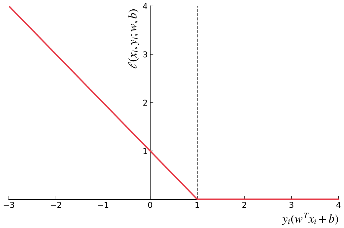
The piecewise linear form of the hinge loss, with a "kink" at $y_i(w^Tx_i+b)=1$.
</figcaption>
</figure>
</div>

<p>Recall that the hinge loss function is defined as</p>

<div id="eq-60">
$$
\ell(x_i,y_i;w,b)={\max(0, 1 - y_i(w^Tx_i+b))} \tag{60}
$$
</div>

<p>At the point where $y_i(w^Tx_i+b)=1$, the hinge loss is nondifferentiable (the “kink”), so there is no unique gradient. However, the subgradient at this point can be either the gradient when $y_i(w^Tx_i+b) &gt; 1$ or the gradient when $y_i(w^Tx_i+b) &lt; 1$ or any value in between. The subgradient of the hinge loss with respect to model parameter $w$ is given by</p>

<div id="eq-61">
$$
{\nabla}_{w}\ell(x_i,y_i;w,b)= \begin{cases}
-y_ix_i &amp;\quad \text{if } y_i(w^Tx_i+b) &lt; 1 \\
0 &amp;\quad \text{otherwise}
\end{cases}
\tag{61}
$$
</div>

<p>and the subgradient with respect to $b$ is given by</p>

<div id="eq-62">
$$
\frac{\partial}{\partial b}\ell(x_i,y_i;w,b)= \begin{cases}
-y_i &amp;\quad \text{if } y_i(w^Tx_i+b) &lt; 1 \\
0 &amp;\quad \text{otherwise}
\end{cases}
\tag{62}
$$
</div>

<p>Therefore, the subgradient of the cost function with respect to $w$ is given by</p>

<div id="eq-63">
$$
\nabla_{w}J(w,b) = \lambda w + \frac{1}{M}\sum_{i=1}^{M}\begin{cases}
-y_ix_i &amp; \text{if } y_i(w^Tx_i+b) &lt; 1 \\
0       &amp; \text{otherwise}
\end{cases}
\tag{63}
$$
</div>

<p>and the subgradient with respect to $b$ is given by</p>

<div id="eq-64">
$$
\frac{\partial}{\partial b}J(w,b)=\frac{1}{M}\sum_{i=1}^{M}\begin{cases}
-y_i &amp; \quad \text{if } y_i(w^Tx_i+b) &lt; 1 \\
0    &amp; \quad \text{otherwise}
\end{cases}
\tag{64}
$$
</div>

<p>For each iteration $t$, the subgradient descent update rule for minimizing the cost function $J(w,b)$ is defined as</p>

<div id="eq-65">
$$
\begin{aligned}
w_{t+1} &amp;\leftarrow w_{t} - \eta \nabla_{w}J(w_t,b_t) \\
b_{t+1} &amp;\leftarrow b_{t} - \eta \frac{\partial}{\partial b}J(w_t,b_t) 
\end{aligned}
\tag{65}
$$
</div>

<p>where $0&lt;\eta&lt;1$ is the learning rate.</p>

<!-- Now, we can directly optimize the primal SVM objective using stochastic subgradient descent. Check out the notebook for implementation: -->
<p>We are now ready to apply stochastic subgradient descent to optimize the primal soft-margin objective. Check out the notebook for implementation:</p>

<div>
  <a class="repo-card" href="https://github.com/jdx/mise" target="_blank" rel="noopener noreferrer">
    <span class="repo-card__header">
      <span class="repo-card__name">jdx/mise</span>
      <svg class="repo-card__github" viewBox="0 0 24 24" aria-hidden="true" focusable="false">
        <path d="M12 .297a12 12 0 0 0-3.793 23.385c.6.111.82-.261.82-.577v-2.234c-3.338.726-4.043-1.416-4.043-1.416-.546-1.387-1.333-1.756-1.333-1.756-1.09-.745.083-.729.083-.729 1.205.084 1.839 1.237 1.839 1.237 1.07 1.835 2.807 1.305 3.492.998.108-.776.419-1.305.762-1.605-2.665-.303-5.467-1.334-5.467-5.931 0-1.31.469-2.381 1.236-3.221-.124-.303-.535-1.524.117-3.176 0 0 1.008-.322 3.301 1.23a11.52 11.52 0 0 1 6.006 0c2.291-1.552 3.297-1.23 3.297-1.23.654 1.652.243 2.873.119 3.176.77.84 1.235 1.911 1.235 3.221 0 4.609-2.807 5.625-5.479 5.922.43.372.823 1.102.823 2.222v3.293c0 .319.216.694.825.576A12.001 12.001 0 0 0 12 .297Z" />
      </svg>
    </span>
    <span class="repo-card__description">Support Vector Machines from First Principles.</span>
    
    <span class="repo-card__languages">
      <span class="repo-card__language" style="--language-color: #da5b0b;">Jupyter Notebook</span>
    </span>
    
  </a>
</div>

<div id="5-closing-thoughts"></div>

<h2 id="5closing-thoughts">5  Closing thoughts</h2>

<p>SVMs are a vast topic, and if some of the concepts take a few readings to sink in, that’s okay. Nobody absorbs all the details in one read.</p>

<p>If this all makes sense, you should now have a pretty good mental model of how SVMs work intuitively, and the mathematics behind them should feel less like a pile of formulas to memorize and more like a series of choices you might have made yourself.</p>

<p><em>If you found this post helpful, consider sharing it with someone who might benefit from it!</em></p>

<p>If you like this type of content and want to learn more or spot any errors in the post, make sure to reach out to me on <a href="https://x.com/gordic_aleksa">X</a> or <a href="https://www.linkedin.com/in/aleksagordic/">LinkedIn</a>.</p>

<p>That’s all for now, thanks for reading!</p>]]></content><author><name>Didarul Islam</name></author><category term="Machine learning" /><category term="Optimization Theory" /><category term="Kernel Methods" /><summary type="html"><![CDATA[Support Vector Machines (SVMs) were first proposed by Vladimir Vapnik and Alexey Chervonenkis in the mid-1960s and have since evolved into one of the most flexible and effective machine learning tools available [8]. At their core, SVMs rest on some genuinely beautiful mathematics, and in this post, we’ll walk through it together in manageable pieces. This post aims to be self-contained: detailed enough that you can learn about the topic in its entirety without juggling multiple resources, yet concise enough so you can avoid the trap of minutiae.]]></summary></entry></feed>